Computing Free Energy Surfaces
Estimating from Samples: Ergodicity
Computing an FES from Eq. eq:FES requires estimating the marginal equilibrium distribution , typically estimated from molecular dynamics or Monte Carlo trajectories. This estimate assumes ergodicity, hence implying that sufficiently long trajectories sample phase space according to equilibrium weights, making time averages equivalent to ensemble averages. Formally, for an observable :
where is the canonical distribution, is the potential energy, and the configurational partition function. In the specific case of a collective variable , the ergodic hypothesis ensures that the empirical distribution of obtained from sampling, converges to equilibrium in the long-time limit:
When systems feature metastable states separated by high barriers, unbiased simulations on practical timescales often fail to achieve ergodic sampling, leading to incomplete estimates of ; enhanced sampling methods address this by accelerating rare transitions, ensuring thorough exploration of relevant states, and yielding reliable FESs that capture both thermodynamic stability and kinetic accessibility.
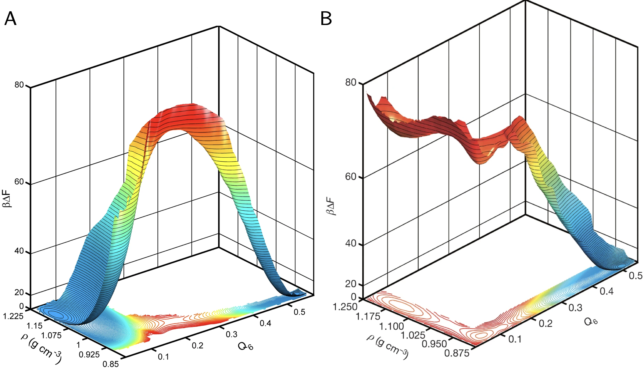
Figure 1:Discovering and Mapping Elusive Metastable Phases of Water. Two FESs at different T and P for the ST2 model of water. A. The FES shows the coexistence between liquid water and ice Ih at 2.6 kbar and 275 K. Ice and water are in equilibrium, hence their respective FES minima have the same depth. B. FES in conditions where Ice is stable, and liquid water is metastable (228.6 K, 2.4 kbar). Interestingly, liquid water in these conditions is characterized by two local minima at low and high density (Poole et al. 1992; Palmer et al. 2014; Gallo et al. 2016). In their landmark study, Palmer et al. used six complementary sampling and Free Energy calculations techniques to demonstrate that the two liquids are separated by a 4 barrier, with finite-size scaling indicative of a first-order transition. At the same time, both remain metastable relative to cubic ice. Figure reproduced with permission from(Palmer et al. 2014).
Recovering Ergodicity via Biased Sampling: Foundations
Biased enhanced sampling methods aim to efficiently achieve ergodicity by introducing an artificial bias potential that modifies the system Hamiltonian,
to alter the equilibrium distribution into a biased one . Reweighting techniques, often rooted in Zwanzig’s free energy perturbation Zwanzig, 1954, enable the recovery of unbiased distributions. Building on these principles, methods such as Umbrella Sampling, Blue Moon Ensemble, and Metadynamics enable the computation of FESs from biased ensembles; for a comprehensive overview, see Ref. Hénin et al., 2022.
Free Energy Perturbation and Thermodynamic Integration
The term Free Energy perturbation (FEP) describes a series of methods originating in the thermodynamic perturbation (TP) one, which evaluates the free-energy change when switching from a reference Hamiltonian to a perturbed one via Zwanzig’s formula Zwanzig, 1954,
where the subscript 0 is a reminder that the average has to be taken using the unperturbed Hamiltonian to integrate the equations of motions. The formula is exact for any value of , so the term “perturbation” is somewhat misleading. However, the sampling is efficient only when configurations sampled under overlap well with those favored by . Stratifying the jump into neighboring states gives multistep TP,
The principle of TP is at the core of numerous methods described in the following sections.
Thermodynamic Integration
Thermodynamic integration (TI) is in effect an application of multistep TP in the limiting case of infinitesimally small changes:
Eq. eq:TI can be rigorously derived from Eq. eq:multiTP using the first term of the cumulant expansion Kubo, 1962
, or by integrating .
The TI formula has a precise interpretation as the integral of the
generalized mean force; however, one needs to take care to ensure the
quasi-adiabatic limit. In fact, the early single-configuration TI (SCTI)
implementation replaced the ensemble average by a single instantaneous
value taken while changing continuously but showed hysteresis Mitchell & McCammon, 1991 at finite switching rates , a clear
sign of non-equilibrium. Multiconfiguration TI (MCTI) Straatsma & McCammon, 1991 addresses this issue by calculating proper ensemble
averages at each value of , yielding per-window statistical errors,
and is also an embarrassingly parallel algorithm. Despite the
development of more efficient methods, the flaw of implementing a
non-equilibrium sampling has sparked new interest in SCTI in the context
of Jarzynski’s identity and steered molecular dynamics Hummer, 2001Park & Schulten, 2004, see Section
sec:single
When the perturbation affects an internal CV rather than an interaction parameter, the system has to be kept at or in the vicinity of the chosen value of . If the configuration change is driven by a -dependent perturbation in the form of a restraint , typically a harmonic potential, the free energy of the unrestrained system is recovered by unbiasing the TI result with TP of the restraint Straatsma & McCammon, 1991:
Another way of looking at the TI when the RC is a function of atomic coordinates instead of a parameter of the Hamiltonian, for example . In this case the PMF along the RC in terms of the conditional probability is written as
The free energy difference takes the form
where the conditional average is defined by
This can easily be recovered as the stiff limit of a harmonic restraint. In the case of holonomic constraints being imposed rather than restraints, correct unbiasing requires more complex approaches described in Sec.sec:BM.
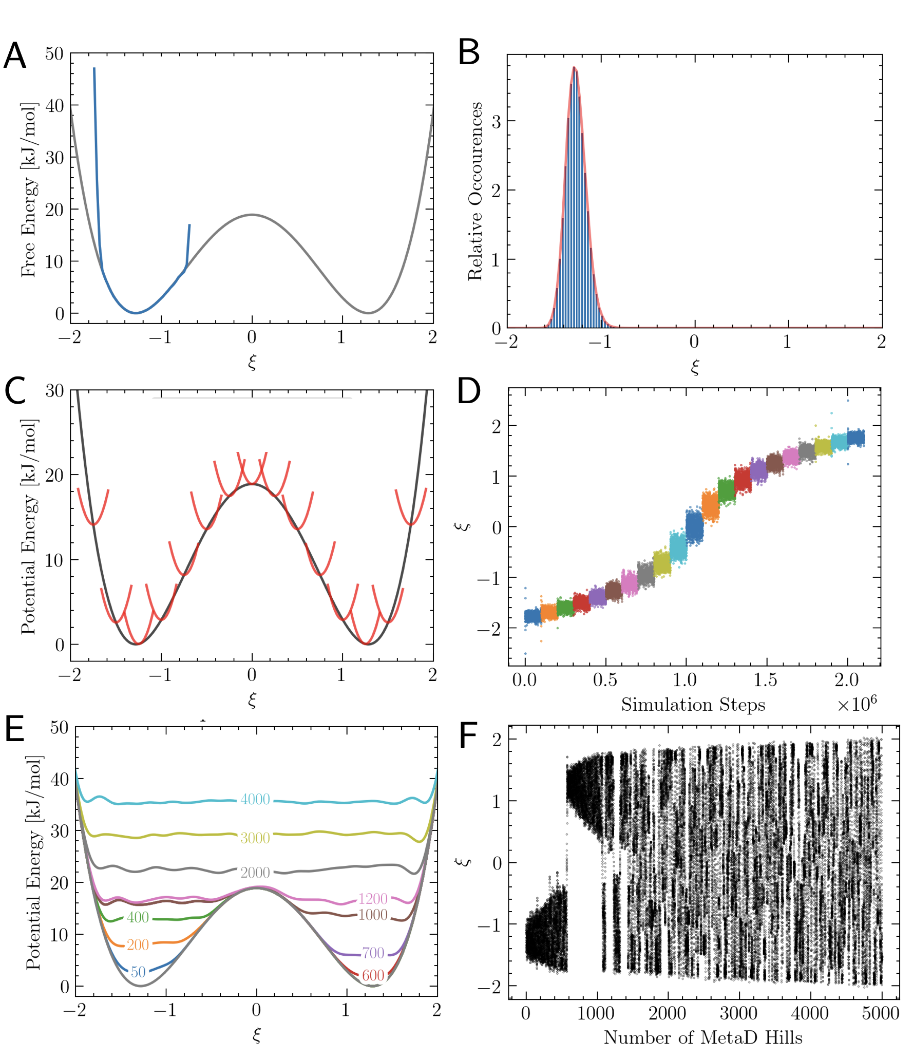
Figure 2:Overcoming sampling limitations with biased approaches A, B. Unbiased simulations. When high free energy barriers hinder transitions between metastable states, only local estimates of are accurate. C, D. Umbrella Sampling. In US multiple restrained simulations centered at reference positions (red parabolas in C), enable a uniform coverage of the reaction coordinate, shown in D; the sampled biased histograms are subsequently combined to recover the full free energy profile (see Sec. sec:UmbrellaSampling). E, F. Metadynamics In MetaD, the bias is history-dependent, progressively filling free energy wells and promoting barrier crossing. The dynamics of , under the effect of bias (panel F) shows how an ergodic exploration of configuration space is associated with bias construction (see Sec. sec:metadynamics).
Umbrella Sampling
Umbrella sampling (US), introduced by Torrie and Valleau in the 1970s Torrie & Valleau, 1977Kästner, 2011, is one of the earliest enhanced-sampling methods to compute an FES along a CV . US is a static bias method, i.e., the biasing potential does not change in time. The central idea of US is to overcome the poor sampling of high-energy regions by introducing a ---usually harmonic--- restraint, which localizes the sampling around a reference value :
In the context of TP, can be seen as the perturbation introduced in the physical Hamiltonian of the system in each of the simulations.
In US, a series of such biased simulations (“windows”, Fig. fig:biasedC) is performed to span the full range of (see Fig. fig:biasedD). Each window produces a biased distribution . The unbiased distribution in window is formally recovered as
from which the free energy (or potential of mean force, PMF) is obtained using Eq. eq:FES. Because each window only samples a narrow range of , the problem of stitching the windows together arises: the free-energy offsets between windows are not known directly.
Several post-processing strategies exist, all rooted in FEP and TI concepts Roux, 1995. The Weighted Histogram Analysis Method (WHAM) Kumar et al., 1992 is the de facto standard post-processing tool in umbrella sampling and determines the free-energy offsets self-consistently by minimizing statistical error, merging all biased histograms into a single distribution (see also Souaille & Roux, 2001Hub et al., 2010. The Multistate Bennett Acceptance Ratio (MBAR) method provides an equivalent, statistically optimal alternative to WHAM Shirts & Chodera, 2008Tan et al., 2012.
An alternative that avoids explicit offset estimation is umbrella integration (UI) Kästner & Thiel, 2005, which reconstructs the mean force directly from the biased distribution,
yielding the PMF by integration over . This way, UI makes explicit the proximity between US and thermodynamic integration methods, effectively implementing an FES estimator similar to Eq. eq:TI_gen We note that UI inspired the development of Mean Force Integration, which can be applied to the post-processing of sampling gathered with both static and adaptive biasing methods Marinova & Salvalaglio, 2019Bjola & Salvalaglio, 2024F. et al., 2024.
Overall, umbrella sampling can be viewed as a restrained-sampling framework analyzed either by histogram reweighting (WHAM/MBAR) or by mean-force integration (UI); both approaches converge to the same PMF given sufficient sampling.
Over the years US has inspired many extensions. Adaptive US iteratively refines the bias toward uniform sampling Mezei, 1987, while local elevation US introduces a history-dependent bias reminiscent of early metadynamics Huber et al., 1994Hansen & Hünenberger, 2010Laio & Parrinello, 2002. Multidimensional formulations Bartels & Karplus, 1997Kästner, 2009 treat coupled coordinates, and hybrid schemes, such as self-learning adaptive variants Wojtas-Niziurski et al., 2013 or replica-exchange US Jiang et al., 2012, enable efficient, massively parallel implementations. These developments confirm US remains a versatile and widely used framework for free-energy calculations.
Constrained reaction coordinates: the Blue Moon Ensemble
Often, holonomic constraints, where the constraining force acts along Goldstein et al., 2014Van Kampen & Lodder, 1984, are used as an alternative to harmonic restraints to enforce a specific value of the CV using algorithms like SHAKE Ryckaert et al., 1977. In this case, one needs to apply an unbiasing factor to correct for momentum loss along the constraint Carter et al., 1989. Combining this factor with the contribution from the integration over (all, including the unbiased) kinetic degrees of freedom yields the Blue Moon ensemble configurational formula (so named because it helps sample events that happen “once in a blue moon”)
where is the mass-metric tensor appearing in Eq.
eq:metric
Adaptive Bias Methods: Metadynamics and derived methods
A key ingredient of US is the use of a fixed set of windows chosen a priori, with convergence depending on their overlap. A complementary class of methods instead builds the bias adaptively as the simulation progresses. Metadynamics (MetaD), introduced by Laio and Parrinello Laio & Parrinello, 2002, is one of the most influential adaptive-bias algorithms for reconstructing FESs Barducci et al., 2011Laio & Parrinello, 2002Bussi & Laio, 2020Valsson et al., 2016. Its central idea is to discourage a molecular simulation from revisiting previously explored regions of the space of CVs ; in doing so, metadynamics enhances the fluctuations along , thus speeding up the sampling Valsson et al., 2016. A MetaD simulation evolves under a time-dependent bias potential that is incrementally constructed as the trajectory progresses. At regular time intervals, a small repulsive Gaussian hill of height and width is deposited at the instantaneous CV value :
This “computational sand-filling” Barducci et al., 2011 progressively raises the free-energy of ensembles of configurations visited during sampling, allowing the system to escape local minima and visit new regions of phase space. In the long-time limit, the accumulated bias offsets the underlying free-energy surface up to an additive constant, so that . Once this condition is reached, the biased dynamics samples a uniform probability distribution in CV space, effectively restoring ergodicity (see Sec. sec:Theory).
MetaD is conceptually related to other history-dependent approaches, such as the local elevation method Huber et al., 1994. In particular, MetaD shares with local elevation the general principle of discouraging revisits to previously explored regions of collective variable space, while differing in its formulation and bias-update protocol. Moreover, compared with earlier mean-force-based schemes such as the Adaptive Biasing Force (ABF) method Comer et al., 2015Darve & Pohorille, 2001Darve et al., 2002, metadynamics constructs the bias from local visitation history rather than explicit force estimates. Despite its simplicity and general applicability, MetaD suffers from a few drawbacks: the continual deposition of Gaussians can lead to systematic overshooting of the free-energy surface; convergence depends on the choice of Gaussian height and width; and the time dependence of complicates rigorous reweighting. These issues motivated the development of statistically controlled variants that address these shortcomings Barducci et al., 2008Valsson et al., 2016Bussi & Laio, 2020.
Well-tempered metadynamics Barducci et al., 2008, is the most popular variant of metadynamics that addresses several of these issues. For instance, WTMetaD introduces a smooth tempering of the bias deposition rate to achieve self-limiting convergence. This is achieved by imposing a dynamic evolution of the Gaussian heights that decreases exponentially with the local value of the bias already accumulated:
where is the bias factor. At the beginning of a simulation, the Gaussian bias height is ; as grows, the added bias diminishes, so that asymptotically approaches a smoothed version of the underlying FES as . The bias factor tunes the trade-off between exploration (large ) and accuracy (small ). The stationary distribution sampled by WTMetaD in the long-time limit is no longer flat but well-tempered, i.e. . The sampling along therefore occurs at an effectively elevated temperature , which thus enhances barrier crossing while maintaining a known, analytically recoverable bias. WTMetaD has, de facto, become the standard formulation implemented in modern software (e.g., PLUMED Tribello et al., 2014, GROMACS Lindahl et al., 2022, LAMMPS Thompson et al., 2022) because it provides controlled convergence, improved statistical efficiency, and the possibility to monitor the flattening of the free-energy landscape on-the-fly.
One can combine WTMetaD with static biases (e.g., harmonic restraints, walls, or custom static biases) in a straightforward, additive manner @Awasthi2016, Limongelli et al., 2013, @MFI_Bjola. If the WTMetaD bias is deposited sufficiently slowly - so that transition states remain effectively bias-free - the infrequent metadynamics framework allows barrier-crossing times to be rescaled to recover physical rate constants Tiwary & Parrinello, 2013Salvalaglio et al., 2014Palacio-Rodriguez et al., 2022. The bias potential accumulated during a MetaD or WTMetaD simulation modifies the underlying probability distribution, so that direct estimates of the free energy from the bias are inherently time-dependent. Several formulations have been proposed to obtain time-independent free-energy estimators, which recover or the distribution of other observables from a trajectory sampled under the effect of a time-dependent bias Tiwary & Parrinello, 2015Bonomi et al., 2009Marinova & Salvalaglio, 2019Giberti et al., 2019Ono & Nakai, 2020.
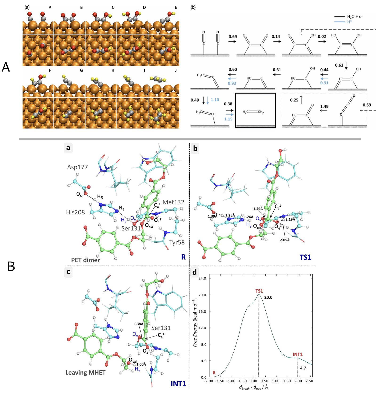
Figure 3:Free energy landscapes of reactions in complex systems
A. A landmark use of metadynamics for reaction discovery from Cheng
et al. on CO reduction on copper (Cheng, Xiao, and Goddard III 2017).
Using ab initio molecular dynamics with explicit water and Blue Moon
refinement, they computed atomistic free-energy barriers and pathways.
At moderate potentials (U > --0.6 V vs RHE, pH 7), ethylene dominates
via CO--CO coupling in an Eley--Rideal step (
eV), while at more negative potentials hydrogen blocks sites, favoring
methane formation through a CHO intermediate. The study offers a
mechanistic basis for tuning Cu-based catalysts in electrochemical
CO reduction. B. A recent example of the traditional use of US
is the study of the catalytic mechanism of PETase by Jerves et
al.(Jerves et al. 2021), providing the first quantitative free-energy
description of PETase catalysis by mapping the full reaction cycle with
QM/MM US. Despite the absence of more modern collective-variable
discovery tools, the study showed that chemical insight can guide the
selection of effective CVs. The FE profile reproduced experimental
barriers (20.0 kcal/mol vs. 18--19 kcal/mol measured) and revealed a
concerted, tetrahedral transition state mechanism distinct from earlier
proposals.
Recent developments have further generalized ideas originating from metadynamics by recasting bias construction in probabilistic or variational terms, giving rise to methods such as Variationally Enhanced Sampling (VES) Valsson & Parrinello, 2014, On-the-fly Probabilty Enhanced Sampling (OPES) Invernizzi et al., 2020, and GAMBES Debnath & Parrinello, 2020 which differ in how the target distribution is enforced. VES does so by minimizing a KL-based variational functional. In contrast, OPES achieves it via an explicit on-the-fly estimate of the marginal biased probability density and a reweighting-based update of the bias; GAMBES, instead, reconstructs the bias from a Gaussian Mixture approximation of the sampled probability distribution. We refer the reader interested in additional details to the comprehensive review of Henin et al. Hénin et al., 2022.
Free Energy Profiles and Equilibrium Constants
Free energy profiles and PMFs link probabilities to partition functions, allowing computation of equilibrium constants for binding reactions. Care must be taken when connecting to standard free energies, as equilibrium constants in statistical mechanics depend on the reference concentration and are dimensionless, while experimental values refer to M. To avoid confusion, here we refer to the (concentration-based) mass action equilibrium constant using the symbol . For association reactions , the mass action law gives
but this holds only in the thermodynamic limit. In finite simulation boxes containing one receptor and one ligand, the equilibrium constant is instead expressed through the ratio of Boltzmann probabilities for bound and unbound states De Jong et al., 2011:
where is the box concentration, and volume change effects are neglected. Writing , the corresponding mass action equilibrium constant becomes . Roux proposed an equivalent form using a delta function to fix the ligand in bulk Woo & Roux, 2005Roux et al., 2008. Gilson et al. derived the same constant from activities for a rigid ligand,
where the term arises from rotational integration, are symmetry numbers, and the solvent partition function. The contribution coming from volume changes is spelled out explicitly, and the infinite dilution identity has been used. This formulation underpins the double--decoupling method (DDM), in which the ratio of partition functions is obtained by decoupling the ligand at the binding site and in the bulk. Boresch et al. introduced a minimal set of six restraints (one distance , two angles , and three dihedral angles ) to restore the free energy cost of decoupling. The correction is expressed in terms of the respective equilibrium distance , angles , and force constants , and , as
The DDM thus provides a general alchemical framework - encompassing confine-and-release variants - whose rigor relies on the proper application and unbiasing of restraints Gilson et al., 1997Bian et al., 2025.
Reaction Paths on Free Energy Landscapes: Transition Path Sampling
As mentioned in Sec.sec:kinetics, FEPs can be used to extract useful information about reaction kinetics, but care must be taken in presence of complex landscapes. A complementary class of approaches focuses on determining representative transition pathways by optimizing geometric or variational principles. Across these families of methods, algorithms inspired by minimum‐action geometry - such as Nudged Elastic Band and its extensions [Jónsson et al. (1998); Henkelman & Jónsson (2000);wang2016automated; Ásgeirsson et al. (2021)] as well as finite-temperature string approaches [weinan2002string; weinan2005finite; E et al. (2007)] and Onsager-Machlup formulations Onsager & Machlup, 1953Adib, 2008Faccioli et al., 2006 - contrast with flux-based kinetic formalisms such as the Bennett-Chandler theory [Ruiz-Montero et al. (1997); Maragliano et al. (2006); vanden2010transition] in that the former determine representative transition pathways by extremizing geometric or variational principles, whereas the latter quantify reaction rates through time-correlation functions and dynamical recrossing statistics.
These geometric and variational approaches provide valuable insight into likely pathways, but a complete statistical description of rare events requires sampling full reactive trajectories, as achieved by Transition Path Sampling (TPS). For a Markovian dynamics, the probability density of a trajectory is
where is the equilibrium distribution and the conditional propagator Bolhuis et al., 2002. The probability that a trajectory initiated in reaches at time is
with
where is the probability of a trajectory to start from , regardless of where it ends at time , and that to start in and end in . These probabilities are expressed in terms of path integrals, effectively functional integrals over the set of all possible paths Feynman, 1948Kleinert, 2009Seifert, 2012. The rate constant, for example, follows from the long-time derivative Bolhuis et al., 2002,
and the problem of evaluating the rate reduces to sampling the path ensemble in the same conceptual way as equilibrium properties are obtained from the Boltzmann distribution.
One can generate trajectories that sample the biased probability of starting in region and ending in region without recrossing in a straightforward manner. Starting from one reactive path, new trial trajectories are generated by small stochastic modifications and integrated forward and backward in time, accepting or rejecting the new path using a Metropolis scheme Metropolis & Ulam, 1949Kalos & Whitlock, 2008Frenkel & Smit, 2023. In the microcanonical ensemble or other generalized ensembles with extended Hamiltonians, the acceptance probability becomes remarkably simple Dellago et al., 2002 as all reactive proposals are accepted. Quantities like the rate are not directly accessible as they are computed with a normalization factor over the path starting in and ending at any point. However, TPS provides direct access to the transmission function via . The rate constant can be accessed by supplementing TPS with a US in the TPE Dellago et al., 1999. Sampling the TPE enables a straightforward computation of the committor function (see Sec.sec:committor). With TPS one can easily identify transition-state configurations by launching short trajectories from frames along the generated paths and selecting those for which .
Related path-sampling approaches include Transition Interface Sampling (TIS) Van Erp et al., 2003Van Erp & Bolhuis, 2005 Forward Flux Sampling (FFS) Allen et al., 2009, and Markov State Models (MSMs) Prinz et al., 2011Chodera & Noé, 2014.
TIS introduces a hierarchy of interfaces between and , estimating the rate as the product of conditional crossing probabilities and the initial flux. FFS instead propagates trajectories forward across interfaces, making it suitable for non-equilibrium or irreversible systems. MSMs reconstruct long-time kinetics from short unbiased trajectories by estimating transition probabilities between metastable states, with rates and committors derived from the transition matrix.
Further refinements include Precision, S-, and Aimless Shooting Grünwald et al., 2008Menzl et al., 2016Peters & Trout, 2006, and hybrid schemes combining TPS with metadynamics or replica exchange Borrero & Dellago, 2016Van Erp, 2007. A detailed overview is given in Bolhuis & Swenson, 2021.
FESs from experiments: single molecule force spectroscopy
Single-molecule force spectroscopy (SMFS) methods---such as AFM and optical or magnetic tweezers---enable experimental probing of molecular free-energy landscapes. A molecule is stretched between a surface and a probe applying controlled force or displacement, with the extension serving as the reaction coordinate. The resulting mechanical response encodes the potential of mean force , recoverable from nonequilibrium work measurements via statistical--mechanical relations. A central theoretical foundation of this connection is Jarzynski’s equality Jarzynski, 1997, which relates nonequilibrium work to equilibrium free-energy differences:
where is the external work performed along the pulling trajectory, and denotes an average over many repetitions of the process. Remarkably, Eq. eq:Jarzynski holds even for transformations driven arbitrarily far from equilibrium, providing a formal bridge between dynamical experiments and equilibrium thermodynamics. Hummer and Szabo Hummer & Szabo, 2005, extended this result to the reconstruction of a full free-energy profile along the molecular extension coordinate , obtaining
where is the time-dependent external potential applied during pulling. For instance, in optical-tweezer or AFM experiments, a harmonic trap of stiffness is displaced at constant velocity , .
Equation eq:HummerSzabo enables reconstruction of the equilibrium free-energy profile from nonequilibrium pulling trajectories. In the adiabatic limit, the work equals the reversible , but real experiments require averaging over many trajectories to account for stochastic fluctuations. Liphardt et al. Liphardt et al., 2002 first validated this approach, showing RNA hairpin unfolding reproduced equilibrium free energies with sub- accuracy. These combined experimental--computational approaches reveal intermediates and barriers, extending free-energy surface reconstruction into the experimental domain through nonequilibrium work theorems.
- Zwanzig, R. W. (1954). High-Temperature Equation of State by a Perturbation Method. I. Nonpolar Gases. J. Chem. Phys., 1420–1426. 10.1063/1.1740409
- Hénin, J., Lelièvre, T., Shirts, M. R., Valsson, O., & Delemotte, L. (2022). Enhanced Sampling Methods for Molecular Dynamics Simulations. ArXiv Prepr. ArXiv220204164. 10.48550/arxiv.2202.04164
- Kubo, R. (1962). Generalized Cumulant Expansion Method. J. Phys. Soc. Jap., 17(7), 1100–1120. 10.1143/jpsj.17.1100
- Mitchell, M. J., & McCammon, J. A. (1991). Free Energy Difference Calculations by Thermodynamic Integration: Difficulties in Obtaining a Precise Value. J. Comput. Chem., 12(2), 271–275. 10.1002/jcc.540120218
- Straatsma, \relax TP, & McCammon, \relax JA. (1991). Multiconfiguration Thermodynamic Integration. J. Chem. Phys., 95(2), 1175–1188. 10.1063/1.461148
- Hummer, G. (2001). Fast-Growth Thermodynamic Integration: Error and Efficiency Analysis. J. Chem. Phys., 114(17), 7330–7337. 10.1063/1.1363668
- Park, S., & Schulten, K. (2004). Calculating Potentials of Mean Force from Steered Molecular Dynamics Simulations. J. Chem. Phys., 120(13), 5946–5961. 10.1063/1.1651473
- Torrie, G. M., & Valleau, J. P. (1977). Nonphysical Sampling Distributions in Monte Carlo Free-Energy Estimation: Umbrella Sampling. J. Comput. Phys., 23, 187–199. 10.1016/0021-9991(77)90121-8
- Kästner, J. (2011). Umbrella Sampling. Wiley Interdiscip. Rev. Comput. Mol. Sci., 1(6), 932–942. 10.1002/wcms.66
- Roux, B. (1995). The Calculation of the Potential of Mean Force Using Computer Simulations. Comp. Phys. Comm., 91, 275–282. 10.1016/0010-4655(95)00053-i
- Kumar, S., Rosenberg, J. M., Bouzida, D., Swendsen, R. H., & Kollman, P. A. (1992). The Weighted Histogram Analysis Method for Free-Energy Calculations on Biomolecules. I. The Method. J. Comput. Chem., 13(8), 1011–1021. 10.1002/jcc.540130812
- Souaille, M., & Roux, B. (2001). Extension to the Weighted Histogram Analysis Method: Combining Umbrella Sampling with Free Energy Calculations. Comput. Phys Comm, 135(1), 40–57. 10.1016/s0010-4655(00)00215-0
- Hub, J. S., De Groot, B. L., & Van Der Spoel, D. (2010). G_wham – a Free Weighted Histogram Analysis Implementation Including Robust Error and Autocorrelation Estimates. J. Chem. Theory Comput., 6(12), 3713–3720. 10.1021/ct100494z
- Shirts, M. R., & Chodera, J. D. (2008). Statistically Optimal Analysis of Samples from Multiple Equilibrium States. J. Chem. Phys., 129(12), 124105. 10.1063/1.2978177
- Tan, Z., Gallicchio, E., Lapelosa, M., & Levy, R. M. (2012). Theory of Binless Multi-State Free Energy Estimation with Applications to Protein-Ligand Binding. J. Chem. Phys., 136(14). 10.1063/1.3701175