
Theory: Defining a Free Energy Surface
Thermodynamic Potentials and Partition Functions
In the canonical ensemble, which describes a system at constant number of particles (), volume (), and temperature (), the probability density of finding the system in a particular microstate characterized by the 6N-dimensional phase space vector of atomic (Cartesian, for simplicity) coordinates and momenta is proportional to the Boltzmann factor , which measures the total energy of the microstate, expressed by the Hamiltonian , in units of the thermal energy , being the Boltzmann constant and the absolute temperature Chandler, 1978Frenkel & Smit, 2023Tuckerman, 2023. The normalization constant of the phase-space density is the partition function , which is, in essence, a Boltzmann-weighted count of the number of accessible microstates and enables a direct connection between molecular configurations (i.e., realizations of ), and thermodynamic concepts familiar to an engineering audience.
The partition function in the canonical ensemble for a system of identical particles is written as:
Two inherently quantum-mechanical terms appear in the normalization factor: the count of permutations of identical particles and the phase space volume unit, , set by the uncertainty principle, which are necessary to obtain an extensive entropy, avoid mixing entropy (Gibbs) paradoxes Noyes, 1961Frenkel & Smit, 2023Tuckerman, 2023 and recover the Sackur-Tetrode entropy of the ideal gas Huang, 1987. Following convention, we will use angular brackets to denote the canonical ensemble average of an observable ,
If the Hamiltonian can be written as the sum of independent kinetic and potential energy terms, , momenta can be integrated out and the partition function can be expressed in terms of the configurational integral
as
where is the thermal wavelength for particles of mass . The configuration (marginal) probability density function is in this case Tuckerman, 2023:
From Partition Functions to Thermodynamic Potentials
The partition function is a central quantity because it encodes all the thermodynamic information of the system in this ensemble. In the canonical ensemble, the thermodynamic potential, known as Helmholtz free energy, , can be written as:
or, in terms of the configuration integral,
where the first term on the right-hand side is the configurational free energy and the second one the translational free energy. Other thermodynamic quantities (i.e., those that depend only on the macroscopic control parameters ) can then be computed as derivatives of . Other statistical ensembles can be derived, for instance, from the canonical ensemble, through a Legendre transformation with respect to one control variable. This operation yields new distribution functions, corresponding to the Laplace transform of the original one. In what follows, we use the symbol to refer to the free energy or thermodynamic potential without connection to an ensemble in particular. The specific meaning of - whether Helmholtz or Gibbs free energy - depends on the statistical ensemble used to sample molecular configurations and compute free energy surfaces, as discussed in Section sec:Computing.
From Thermodynamic Potential to Free Energy Differences
Now, let us consider two disconnected regions of the phase space, and , representing two sets of microstates associated with two distinct states of the system, and . Such ensembles of configurations could correspond to the reactants and products of a chemical reaction, two different phases of the same substance, the unfolded and folded configurations of a biopolymer, etc. By integrating the normalized canonical phase space distribution within (or ), one can obtain the equilibrium probability to observe the system in state (or ), and thus the free energy difference between the two states:
where , are indicator functions selecting only microstates belonging to state , and , respectively. Integrating the indicator functions , ) gives access to the equilibrium probability of states and .
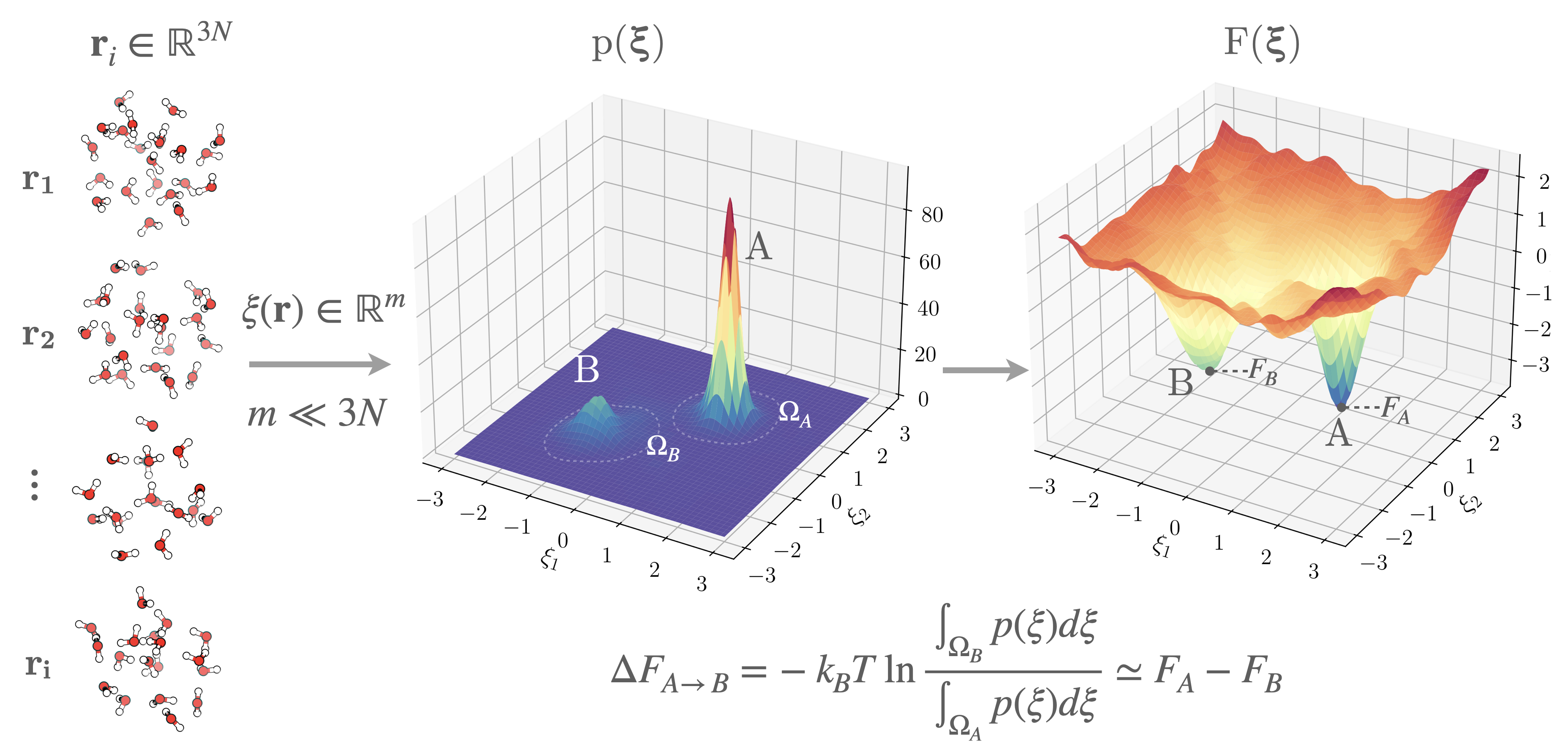
Figure 1:From microscopic configurations to the free energy surface. Each molecular configuration (, where is the number of atoms) is mapped to a point in a reduced space of CVs (), with . The marginal equilibrium probability , which quantifies the relative likelihood of observing configurations consistent with a given value of . The corresponding free energy surface provides a readable map of thermodynamic stability and metastability in configuration space. Basins A and B correspond to metastable states separated by a free energy barrier.
Free Energy Surfaces: readable maps of the thermodynamic potential
Evaluating the equilibrium probability of state , , involves defining the indicator function , which identifies configurations in . Due to the high dimensionality of , this is challenging and typically addressed by introducing a low-dimensional mapping that groups similar microstates and allows defining the marginal equilibrium probability as Kirkwood, 1935Frenkel & Smit, 2023Tuckerman, 2023:
where is the equilibrium probability density of the ensemble of microstates mapping to the same value of . In this context, can be interpreted as the (normalized) partition function associated with all the microstates mapped in . In the following, to favor readability, we indicate as a scalar; however, its dimensionality can be higher than one, and extensions to higher dimensionality are straightforward Laio & Parrinello, 2002Kästner, 2011.
In analogy with Eq.eq:FE we can define a free energy for every as:
where is the FES, and is an arbitrary constant, indicating that is a measure of relative thermodynamic stability between ensembles of states that map to different values of .
Mapping configurations onto a physically meaningful such that, i.e., it captures slow transitions in the configurational ensemble (see Section sec:CVs), renders the features of informative. For instance, for a good choice of , metastable states correspond to local minima in . As a consequence, free energy differences between metastable states become tractable as the domain of integration ( in Eq. eq:DF) can be identified in reduced-dimensionality (see Fig. fig:FES_idea).
A subtle but important point is that FESs are low-dimensional projections of configurational space, where each value of represents an ensemble of possibly distinct microstates whose degeneracy contributes to the configurational entropy Gimondi et al., 2018Dietschreit et al., 2023. Broadly degenerate regions have higher entropy, while narrowly defined ones follow the potential energy more closely. The internal energy contribution to an FES is obtained as a conditional ensemble average over all microstates compatible with the value of :
The entropy surface, then follows from: .
As illustrated in Fig. fig:entropy, basins with identical potential energies can differ in free energy purely due to entropy, an effect crucial in biomolecular and soft-matter systems where conformational transitions and barriers often reflect entropic, rather than energetic, contributions @gimondi2018building, polino2020collective, Kollias et al., 2020, @leanza2023into, @Serse2024.
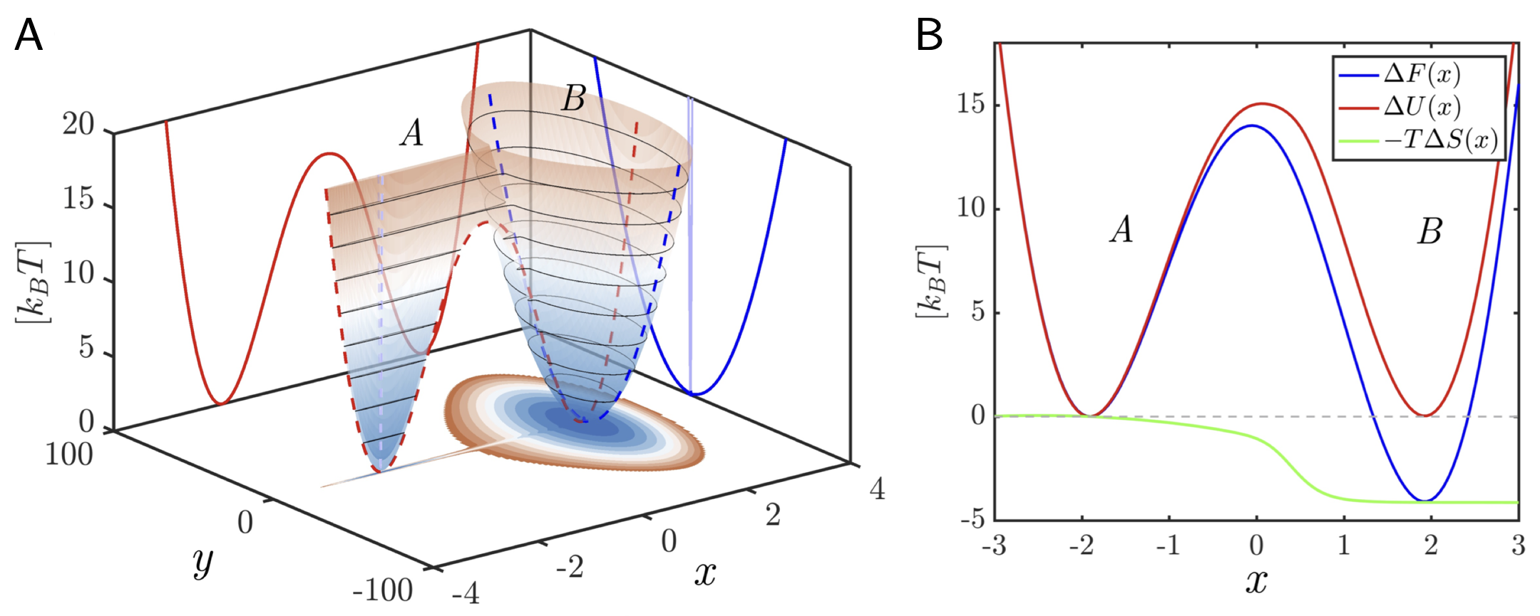
Figure 2:Entropy and Energy surfaces in A. Two-dimensional model potential energy surface, , and corresponding projection on the map variable (x) used to illustrate the decomposition of the free energy surface into energetic and entropic contributions, following Ref. Gimondi et al., 2018. The potential energy landscape features two basins of comparable depth (A and B) but markedly different widths along the coordinate . B. One-dimensional profiles of the free energy (blue), average potential energy (red), and entropic term (green). Although the two minima have identical , basin B exhibits a lower free energy because of its higher degree of configurational degeneracy in , associated with higher entropy. Reproduced with permission from Ref. Gimondi et al., 2018.
Collective Variables, Order Parameters, and Reaction Coordinates
The central role of is to provide a reduced representation of the high-dimensional configuration space that retains the essential ability to distinguish relevant metastable states, and slow transition modes between them, for the molecular process of interest Kirkwood, 1935Frenkel & Smit, 2023, @tuckerman2023statistical. Depending on the field of application, the characteristics of the studied process, and its own properties, the low-dimensional mapping can be referred to by different names. The most common are collective variables (CVs), order parameters (OPs), and reaction coordinates (RCs) Hénin et al., 2022. Although these terms overlap partially and are sometimes used interchangeably by practitioners, they imply some fundamental distinctions. Clarifying and understanding their differences is thus crucial for a consistent interpretation of FESs associated with molecular transformations.
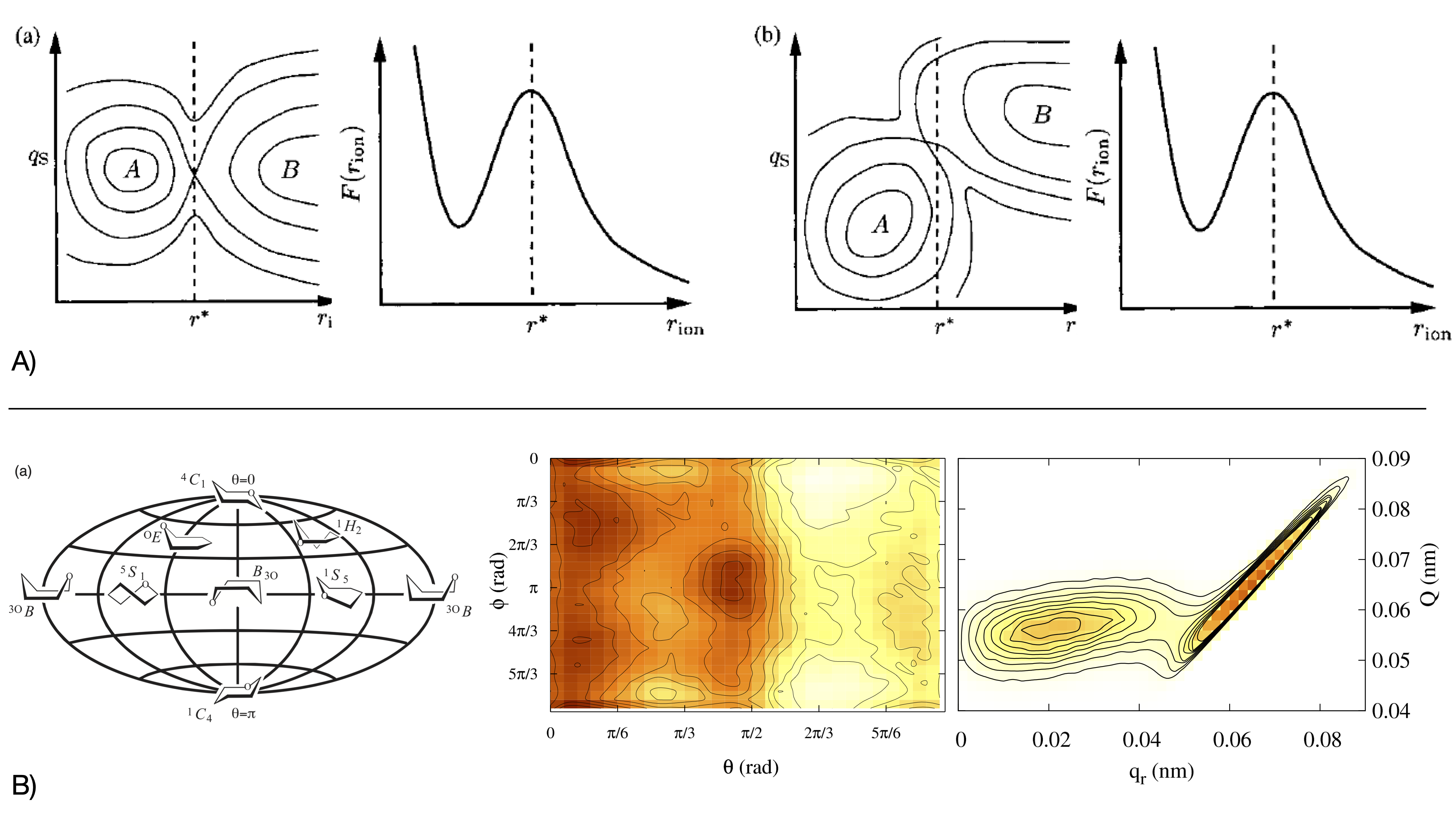
Figure 3:A. Reaction Coordinates and Collective Variables: Lessons from Ion-Pair Dissociation in Water. The distinction between CVs and RCs is both conceptual and practical. An early and historically influential example illustrating this difference is the dissociation of a NaCl ion pair in water, investigated by Geissler et al. Geissler et al., 1999. As illustrated by Geissler, two landscapes with identical projections can imply distinct mechanisms. In the simplest case,(a), the barrier in defines the transition state, making not only a good CV but also a RC. However, when solvent reorganization adds an orthogonal coordinate , b, configurations at belong to stable basins rather than the transition region, so remains a good CV (able to distinguish dissociated from undissociated) but it is not a good RC.
B. Choosing the Right Coordinate: The Ring Puckering Example. The choice of CVs is critical in free-energy calculations, but not always obvious. Puckered ring conformers can be described by the Cremer--Pople Cartesian coordinates, obtained from the out-of-plane displacements of the 6-membered ring atoms as , , , or by their polar representation (left panel). Only are effective variables for biasing, as they capture conformer connectivity. Using two polar coordinates, metadynamics spans the entire puckering free-energy landscape for glucuronic acid (middle panel, 5 kJ/mol isolines), whereas biasing along Cartesian projections fails near the equatorial line. There, ergodicity is broken as the bias acts only perpendicularly to the puckering sphere (right panel). Sega et al., 2009.
Collective Variables and Order Parameters
A CV is the most general of the three denominations: it is any function of the atomic coordinates designed to reduce the enormous dimensionality of a molecular system into a smaller, more interpretable set of descriptors. To be useful, CVs must distinguish all the relevant long-lived metastable states involved in a transformation, i.e., the reactants and the products. In this case, the metastable states of interest will appear as local maxima in , and local minima in the FES, . Typical CVs include simple geometrical descriptors, such as distances and angles Hénin et al., 2022Fiorin et al., 2013Bonomi et al., 2019Tribello et al., 2025, as well as more complex functions, including measures of structural similarity Pietrucci & Laio, 2009 or progress along a path defined by a set of reference structures Branduardi et al., 2007. It should be noted that CVs do not necessarily require a direct physical interpretation, and they can be abstract or highly engineered Pietrucci & Andreoni, 2011. For instance, combinations of distances, angles, or latent variables from dimensionality-reduction algorithms can be effective CVs by allowing for a clear distinction between metastable states Tribello et al., 2012, while losing a direct physical interpretability (see an extended discussion in section sec:MLCVs).
OPs are a specific type of CV introduced in statistical mechanics to distinguish between different thermodynamic phases or states of matter Neha et al., 2022Desgranges & Delhommelle, 2025Giberti et al., 2015. OPs typically reflect a symmetry-breaking or structural feature that changes qualitatively at a phase transition---for example, density in liquid--gas coexistence, orientational alignment in liquid crystals, and roto-translational invariance in crystalline systems Steinhardt et al., 1983Tribello et al., 2017Gimondi & Salvalaglio, 2017Piaggi & Parrinello, 2017. Although OPs are often used to obtain a global description of an atomistic system, they are typically constructed from local contributions within well-defined atomic environments Lechner & Dellago, 2008Bartók et al., 2013Piaggi & Parrinello, 2017Giberti et al., 2015Caruso et al., 2025. When dealing with characterising the state of molecular solids, OPs based on measures of similarity between distributions capturing the translational, orientational, and conformational order are particularly effective Gobbo et al., 2018Gimondi & Salvalaglio, 2017Francia et al., 2020.
Reaction Coordinates
An RC implies a further specialization: it is a low-dimensional descriptor intended to capture the progress of the most probable transition pathway between reactants and products. An ideal RC is not only correlated with the transition but also uniquely parameterizes the progress of the reaction and identifies the transition state ensemble Vanden-Eijnden, 2006Peters, 2017Peters & Trout, 2006. An important point to note is that, when (a combination of) CVs provide a good approximation of the RC for a given physical transformation, saddle points in correspond to the projection of the transition state ensemble of configurations associated with that transformation. For configurations belonging to the transition state ensemble, the probability of completing the crossing of the saddle point and committing to the products (see Sec. sec:committor) is narrowly distributed around .
The Committor Function
The committor function , also known as splitting probability, originally introduced by Onsager Onsager, 1938, provides the most rigorous definition of a reaction coordinate for a system evolving from state A to state B. It is the probability that a trajectory starting from configuration , with momenta drawn from equilibrium, reaches B before returning to A. By definition, , and the transition state ensemble corresponds to the isosurface . Iso-committor surfaces partition configuration space into metastable basins, giving a unique dynamical measure of progress along the reaction. Unlike heuristic collective variables, the committor fully determines kinetic observables such as rate constants and reactive fluxes Vanden-Eijnden, 2006. Although computing it exactly is infeasible for high-dimensional systems, it remains a key reference: an ideal reaction coordinate correlates monotonically with and minimizes its variance within isosurfaces. Thus, the committor defines the optimal projection of dynamics---any reduced representation that preserves its distribution across the transition ensemble retains complete kinetic information Geissler et al., 1999, a concept central to both path sampling Bolhuis et al., 2002Van Erp & Bolhuis, 2005 and modern data-driven approaches.
Free Energy Barriers and Generalised Transition State Theory
Once a suitable RC is defined, the free energy surface quantifies the reversible work required to bring the system to a configuration of progress . Minima of identify metastable states (reactants, products), while the maximum along the minimum free-energy path defines the transition state at . The corresponding free energy difference
represents the free energy barrier that the system must overcome to transform from reactants to products, thus opening the door to a kinetic interpretation of the free energy surface. The generalised transition-state theory (TST) links thermodynamics and kinetics by expressing the rate constant as the thermal average of the flux through a dividing surface in configuration space Peters, 2017:
The prefactor represents the average crossing velocity, while the Boltzmann factor gives the equilibrium probability of reaching the transition state. This form follows from the flux-over-population formalism of Hänggi, Talkner, and Borkovec Hänggi et al., 1990, where the rate of barrier crossing is the ratio of the reactive flux to the reactant population ,
Here selects configurations on the dividing surface, retains forward crossings, and is the Boltzmann weight. Assuming equilibration of degrees of freedom orthogonal to , Eq. eq:TSTHanggi reduces to Eq. eq:TSTPeters, linking the rate constant directly to the free-energy profile obtainable with the methods discussed in Sec. sec:Computing. The exponential term is obtained from the simulation, while the prefactor follows from the mean thermal velocity along . The TST formula does not consider barrier recrossing; these are fully included in approaches like the Bennett-Chandler reactive flux Bennett, 1977Chandler, 1978
where and are characteristic functions identifying reactants and products, and the rate is obtained from the plateau value of . This formula and its successive improvements Ruiz-Montero et al., 1997 require an accurate sampling of the transition state and are limited by the necessity to locate it and the assumption of its uniqueness. Where this is not true Vanden-Eijnden, 2006E, Weinan & Vanden-Eijnden, 2010, the bundle of transition paths must be sampled, as discussed in Section sec:tps.
- Chandler, D. (1978). Statistical Mechanics of Isomerization Dynamics in Liquids and the Transition State Approximation. J. Chem. Phys., 68(6), 2959–2970. 10.1063/1.436049
- Frenkel, D., & Smit, B. (2023). Understanding Molecular Simulation: from Algorithms to Applications (3rd ed.). Elsevier. 10.1016/C2009-0-63921-0
- Tuckerman, M. (2023). Statistical Mechanics : Theory and Molecular Simulation. Oxford University Press. 10.1093/oso/9780198825562.001.0001
- Noyes, R. M. (1961). Entropy of Mixing of Interconvertible Species. Some Reflections on the Gibbs Paradox. J. Chem. Phys., 34(6), 1983–1985. 10.1063/1.1731804
- Huang, K. (1987). Statistical Mechanics. John Wiley and Sons.
- Brett, C. M., Frey, J. G., Hinde, R., Kuroda, Y., Marquardt, R., Pavese, F., Quack, M., Stohner, J., & Thor, A. J. (2023). Quantities, Units and Symbols in Physical Chemistry: Abridged Version. Royal Society of Chemistry.
- Allen, M. P., & Tildesley, D. J. (2017). Computer Simulation of Liquids (2nd ed.). Oxford University Press.
- Rowlinson, J. S., & Widom, B. (2002). Molecular Theory of Capillarity. Dover Publications, Inc. 10.1088/0031-9112/34/10/030
- Kittel, C. (2004). Elementary Statistical Physics. Dover. 10.1007/978-3-319-62063-3_2
- Landau, L. D., & Lifshitz, E. M. (1980). Statistical Physics, Part I (3rd ed.). Pergamon Press.
- Kirkwood, J. G. (1935). Statistical Mechanics of Fluid Mixtures. J. Chem. Phys., 3(5), 300–313. 10.1063/1.1749657
- Laio, A., & Parrinello, M. (2002). Escaping Free-Energy Minima. Proc. Nat. Acad. Sci., 99(20), 12562–12566. 10.1073/pnas.202427399
- Kästner, J. (2011). Umbrella Sampling. Wiley Interdiscip. Rev. Comput. Mol. Sci., 1(6), 932–942. 10.1002/wcms.66
- Gimondi, I., Tribello, G. A., & Salvalaglio, M. (2018). Building Maps in Collective Variable Space. J. Chem. Phys., 149(10). 10.1063/1.5027528
- Dietschreit, J. C., Diestler, D. J., & Gómez-Bombarelli, R. (2023). Entropy and Energy Profiles of Chemical Reactions. J. Chem. Theory Comput., 19(16), 5369–5379. 10.1021/acs.jctc.3c00448.s001